Energy

Started on Jan. 10, 2024
SLB is a global technology company that drives energy innovation for a balanced planet. With a global footprint in more than 100 countries and employees representing almost twice as many nationalities, we work each day on innovating oil and gas, delivering digital at scale, decarbonizing industries, and developing and scaling new energy systems that accelerate the energy transition.
Corrosion-related failures represent serious hazardous events and account for more than 25% of overall well failures in the oil and gas industry (Figure 1). Corrosion of steel pipes throughout the years due to extreme conditions in the wellbore can have negative financial consequences, with potential for significant environmental impacts (groundwater contamination, gas leakage, and seepage at the surface). Pipe condition evaluation for well integrity workflows involves corrosion characterization, leak and structural deficiency monitoring, and detection of potential breaks in the pipe. Accurate corrosion detection is important for both operators and service companies to decrease interpretation time, reduce subjectivity in monitoring, and increase overall performance.
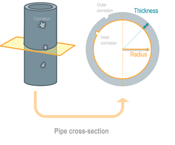
Figure 1 - Corrosion visualization on the well.
Indeed, to inspect steel pipes and detect corrosion along the wellbore, various types of logging imagers are utilized, including electro-magnetic, ultrasonic, and mechanical imagers. These imagers provide granular topographic maps of pipe walls or thicknesses containing information about the pipe's current state such as manufacturing process, collar positions, and defect presence in the pipe's inner or outer wall.
Received pipe thickness images are mappings of the cylindrical-pipe dimensions in polar coordinates. These maps are viewed as 2D images (y-axis being the depth and x-axis the azimuth). THBK is the variation of the thickness around the mean thickness value THAV. The specificity of our data is that it is long (wells can be up to kilometers) and narrow (azimuthal resolution is limited). Due to the telemetry, some processing errors might occur, corrupting some data points on the maps. Therefore, appropriate data cleaning and processing are required before analyzing the data and using them for training as grayscale images (Figure 2).
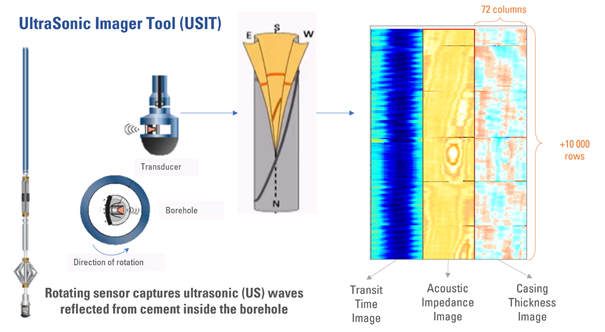
Figure 2 - Ultrasonic Imager Tool; tool sensors and the images obtained.
The goal of the hackathon is to produce a model that gives the highest possible score for groove defect segmentation.
This competition is evaluated on the intersection over union (IoU). The IoU can be used to compare the pixel-wise agreement between a predicted segmentation and its corresponding ground truth. The formula is given by:
$$ \frac{|X\cap Y|}{|X\cup Y|} $$
where $X$ is the predicted set of pixels and $Y$ is the ground truth. The IoU is defined to be 1 when both $X$ and $Y$ are empty. The leaderboard score is the mean of the IoU coefficients for each image in the test set.
The pipes manufactured using a mold represent manufacturing patterns. Manufacturing patterns are homogenous within small sections of the pipes called joints; they are organized in repetitive and visually coherent shapes and forms (circles and horizontal, vertical, or oblique lines with varying thickness). However, intra joint feature distribution is high; two consecutive joints within the same well can have distinctly different manufacturing patterns. These patterns reflect loss and excess of metal due to the manufacturing process.
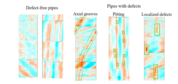
Figure 3. Corrosion and wear defects Examples
Collars are defined as the junction between two joints and are displayed in the radius and thickness map as a line.
Manufacturing patterns and collars represent a background on which defects and anomalies are overlaid. Corrosion in the pipe always appears as metal loss (red patterns in below figure); pipes lose their thickness in the inner or in the outer wall, sometimes simultaneously. (Corrosion is not an either-or process; it may happen on both the inner and outer wall at the same time). Those defects are random in size, metal penetration, and overlay on top of the manufacturing patterns.
Corrosion and wear defects on steel pipes can be classified into three categories:
• Pitting corrosion
• Localized defects
• Axial groove
As mentioned earlier, the database comprises ultrasonic images from 20 wells. Each image within the database is paired with a binary mask of identical dimensions, acting as the corresponding label for that specific image. The well dimensions are outlined as follows:
Train & Validation data:
The images being really big, we already cut them into smaller square patches of size 36x36 pixels. Each image is saved using the following name convention: well_<well_id>_patch_<patch_id>.npy You can load them by using the np.loadfunction.
The labels are binary images of size 36x36, they are saved in a csv file. In order to load them you should read the csv and reshape the labels into the right format.
# Read file
y_train=pd.read_csv(Path('y_train.csv'), index_col=0) #Table with index being the name of the patch

# Access to one patch label
y_train.loc['well_1_patch_130'].reshape(36*36)

# Get all labels at once
y_train.values.reshape((-1,36,36))
Format of the output
The format for the output is a csv where each line is the flatten patch. Here is an example for create the csv file from saved prediction.
from tqdm.auto import tqdm

img_save_dir = Path(f'../data/predictions')
for img_path in tqdm(img_save_dir.glob('*.npy')):
    name = img_path.stem
    if name in labels[phase]:
        continue
    label = np.load(img_path)
    label_tsh = (label>0.5)*1
    labels[phase].update({name:label.flatten()})

pd.DataFrame(labels['Test'], dtype='int').T.to_csv(Path(f'../data/pred.csv'))
The benchmark is established on a simple CNN architecture, meticulously trained on 36x36 patches extracted from the well dataset. At the end of the architecture we added a sigmoid function.
Pre-processing operations were executed to enhance data quality:
The hyperparameters for training were carefully configured:
In contrast, no specific post-processing steps were applied, maintaining the integrity of the model's output.
Files are accessible when logged in and registered to the challenge
Challenge data is supported by: