Challenge context

Variations of the sea level are composed of the tide and the surge.

The tide is composed of the astronomical tide (due to gravitational forces exerted by the Moon and the Sun – other planets being negligible), and the radiational tide (due to meteorological cyclic effects). It is easily predicted.

The surge is the difference between the observed sea level and the tidal predicted sea level (i.e. the tide). The surge can be positive or negative. Its forecast and understanding is of critical importance for safety reasons.

There are two main physical phenomena that cause surges: wind and atmospheric pressure. Wind exerts friction on the water surface, generating a modification of the currents and of the sea level, and hence an accumulation of water when approaching the coastline. On the other hand, atmospheric pressure determines the weight of the air masses above the sea, which in turn decreases (or increases) the sea level mechanically. A decrease (resp. increase) in atmospheric pressure of one hectopascal (hPa) is approximately equivalent to an increase (resp. a decrease) of one centimeter in water level.

In addition, the waves may contribute to increase the storm surges, when they break near the coast. This additional surge due to wave breaking is referred to as “wave setup”. Here, we will focus on data of high water surges, also referred to as “skew surge”.

Tide surges are crucial to forecast

Falling tree due to Xynthia in Darmstadt, Germany

Surge prediction can have crucial impact to mitigate the effects of coastal water submersions. In the case of the Lothar strom in december 1999, the very low pressure linked to the storm (960 to 970 hPa at the heart of the storm) combined with the accumulation of water on the coastline due to the westerly winds, caused remarkable surges of around 70cm to 1m, particularly near the trajectory of the low pressure center (Brittany and Normandy). In the case of the Xhyntia strom in february 2010, the surge reached an exceptional value of nearly 1.5m on the Vendée and Charente coasts, causing drastic floodings that led to severe human casualties and material losses. The ability to accurately predict surges is hence crucial for metorological crisis management.

Damage and flooding following the Xynthia storm in Fouras, Charente-Maritime, France

Challenge goals

Participants will have to forecast the sea surges in two western European coastal cities.

We place ourselves in a forecast setup: knowing the surge values and the sea-level pressure field in the last 5 days, we want to predict the surge values in the next five days. It is hence a time series prediction problem. The signals we consider are:

• the surge, which is a function of the time.
• the sea-level pressure, which is a function of the time, the latitude and the longitude.

The score $\ell(\hat{y}, y)$ we use to measure the quality of the prediction $\hat{y}$ compared to the true values $y$ is a weighted version of the mean square error (MSE). The weights depend linearly on the forecast time, with a bigger weight for the first forecast time and a lower weight for the last forecast time. The prediction for the two cities are computed independently, and the final loss is their sum:

def surge_prediction_metric(y_true, y_pred):
    w = np.linspace(1, 0.1, 10)[np.newaxis]
    surge1_cols = [
        'surge1_t0', 'surge1_t1', 'surge1_t2', 'surge1_t3', 'surge1_t4',
        'surge1_t5', 'surge1_t6', 'surge1_t7', 'surge1_t8', 'surge1_t9' ]
    surge2_cols = [
        'surge2_t0', 'surge2_t1', 'surge2_t2', 'surge2_t3', 'surge2_t4',
        'surge2_t5', 'surge2_t6', 'surge2_t7', 'surge2_t8', 'surge2_t9' ]
    surge1_score = (w * (y_true[surge1_cols].values - y_pred[surge1_cols].values)**2).mean()
    surge2_score = (w * (y_true[surge2_cols].values - y_pred[surge2_cols].values)**2).mean()

    return surge1_score + surge2_score

Since the surge values are normalised (zero mean and standard deviation 1), $1 - \ell$ can be seen as a percentage of explained variance. With a trivial zero prediction of all values, the score is $\ell \approx 1$, meaning that we explain 0 % of the variance. A score bigger than one is hence worse that the zero prediction and can be considered as "bad".

Data description

The training set contains 5599 entries, and the test set contains 509 entries. Each entry represents approximatively 5 days of measurements of the pressure and the tide, and the times at which they were done.

Times are given in the GMT convention. In the GMT convention, the time is expressed as the number of seconds elapsed since January 1st, 1970; they can be converted to the usual Gregorian time with time.gmtime(). Note that in our dataset, some times are negative: indeed, the first measurements date back to the 1950s. For instance, the very first sea-level pressure field is given at $t = -631108800.0$ which corresponds to 1950, January 1st at approximately 21h.

Sea-Level Pressure fields (SLP) are given every three hours, so there are 40 fields for every observation. They cover the Atlantic front of western Europe and Iceland, as shown on the following map: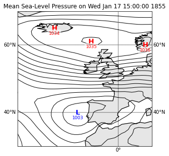 

Sea surges are measured for each high tide, i.e. every 12 hours approximately. We measure the sea surge at two different locations, which are two anonymous European costal cities. Consequently, each entry contains $2 \times 10$ values to predict. There are in total $20 \times 509 = 10180$ values to predict for the test. Note that the surge values in cities 1 and 2 have been normalized, such that they have 0 mean and standard deviation 1. The true means and std of the surge are of the order of 10cm and 20cm respectively.

The .npz format: practically, the input X is encoded in the numpy .npz format and consists of:

• id_sequence: the ids of the sequence
• t_slp: the 40 GMT times at which the sea-level pressure (SLP) fields are given.
• slp: the 40 sea-level pressure (SLP) fields, encoded in images of size (41, 41).
• t_surge1_input: the 10 GMT times at which the surge heights are given in city 1.
• surge1_input: the given surge heights in city 1.
• t_surge2_input: the 10 GMT times at which the surge heights are given in city 2.
• surge2_input: the given surge heights in city 2.
• t_surge1_output: the 10 GMT times at which we must predict surge heights in city 1.
• t_surge2_output: the 10 GMT times at which we must predict surge heights in city 2.

To access for example the training slp, one can use the following:

X_train = np.load('X_train_surge.npz')
slp = X_train['slp']

The output Y is encoded in a csv file with the columns:

• id_sequence: the ids of the sequence
• surge1_t{0...9}: the correct surge height in city 1 at time 0 to 9
• surge2_t{0...9}: the correct surge height in city 2 at time 0 to 9

Submission format We provided a random submission example. The submission index must be X_test['id_sequence'] and the columns must match those of Y_train_surge.csv: see the notebook in the supplementary files for another submission example.

Benchmark description

Analog methods in meteorology are the equivalent of nearest-neighbors predictions in machine learning. It consists in finding a day in the past when the weather scenario looked very similar to the actual weather scenario (an analog scenario). The forecaster would predict that the weather in this forecast will behave the same as it did in the past. Physicists appreciate these methods for their interpretability, as the prediction is explained by a real past situation that they can look at. They can also a posteriori analyze the prediction errors given the difference between the actual scenario and the analog found in the past.

The benchmark we propose here is an analog method. We use the standard L2 metric and look for the closest $k=40$ scenarios at time t and t - 24h using a K-nearest neighbour search. We then average over these scenarios to get the benchmark. It yields a score of 0.77 on the public test data, meaning that it explained around 23 % of the variance.

We provide in the supplementary files a jupyter notebook that implements this benchmark.