Challenge context

Colloids: How small can we go?

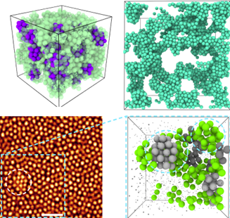
The Royall Group is interested in using nano-colloidal systems to address the glass transition, which is arguably the greatest outstanding challenge in the basic physics of everyday materials. Colloids mimic atoms and molecules and thus exhibit the same behavior, such as forming (colloidal) glasses. However, since they are micron-sized, they can be imaged with 3d microscopy and their coordinates tracked, to test theories of the glass transition (above figure). Smaller colloids enable a more robust test of theoretical predictions, because it is possible to access states where new physics is predicted. To this end, we used a new super-resolution “nanoscopy” to pioneer the imaging of nano-colloids, which reveals new insights into the glass transition. However, if we can use even smaller particles, we expect to learn much more, and for this reason, we wish to develop a machine learning method for 3d tracking of small nano-colloids.

Contact

C. Patrick “Paddy” Royall ESPCI Paris, paddy.royall@espci.fr

Abdelwahab Kawafi, University of Bristol, a.kawafi@bristol.ac.uk

Giulio Biroli, ENS Paris, giulio.biroli@ipht.fr

Challenge goals

Can you detect small particles from a noisy 3D scan?

Problem definition

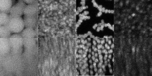
Many applications are used to track spheres in three dimensions. However, the most difficult part of detecting colloids is how densely packed they are. Most methods struggle to detect a majority of the particles, and there is a higher incidence of false detections due to spheres that are touching.

This is defined as the volume fraction ($\phi$ or volfrac for short) and represents the volume of the particles divided by the total volume of the region of interest. Below you can see an image of various real images of colloids at different volume fractions.

Moreover, it is impossible to create manually labelled data for this project since there are thousands of colloids per 3d volume, and more importantly manual labelling would be too subjective. Due to this we have created a simulated training dataset. To reduce photobleaching of the tiny particles during imaging we need to reduce the confocal laser power. This results in a low contrast to noise ratio (CNR). CNR is defined as (see the wikipedia article for more detail):

$$CNR = \dfrac{b_{\mu} - f_{\mu}}{\sigma}$$

where $b_{\mu}$ and $f_{\mu}$ are the background and foreground mean brightnesses, and $\sigma$ is the standard deviation of gaussian noise.

It also contributes to a high signal to noise ratio (SNR) which is simply:

$$SNR = \dfrac{f_{\mu}}{\sigma}$$

In addition to the high SNR and low CNR, this problem has further unique challenges:

• Relatively small training sample size ($n=1400$)
• Relatively large 3D input size ($64 \times 64 \times 64$)
• The final prediction (x_test) will be for larger sizes than the training samples ($128 \times 128 \times 128$)

The figure below shows some of the steps of the simulation:

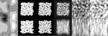The simulation steps are very simple:

1. Background is drawn
2. Foreground (spheres) is drawn
3. The image is blurred
4. The point spread function is convolved
5. Zoom of the previous image
6. Noise is added

Metric

Our metric is average precision (AP). This is similar to ROC and contains information on precision (fraction of correct detections), recall (how many of all particles are detected), as well as distance of the detections from the truth given by the threshold. Almost all available AP implementations are in 2D, but we provide in the supplementary files a script custom_metric.py that will measure this for you in 3D for spheres. Precision is key and is the most crucial factor for good detections, however, the higher the recall the bigger the sample that can be used for downstream analysis.

This example shows how to read x, y, and metadata and analyses precision, recall, and average precision.

from custom_metric import average_precision, get_precision_recall, plot_pr
from read import read_x, read_y
import pandas as pd
from matplotlib import pyplot as plt

index = 0
x = read_x(x_path, index)
y = read_y(y_path, index)
metadata = pd.read_csv(m_path, index_col=0)
metadata = metadata.iloc[index].to_dict()

# Find the precision and recall 
prec, rec = get_precision_recall(y, y, diameter=metadata['r']*2, threshold=0.5)
print(prec, rec) # Should be 1,1
# Find precision and recall of half the positions as prediction
prec, rec = get_precision_recall(y, y[:len(y)//2], diameter=metadata['r']*2, threshold=0.5)
print(prec, rec) # Should be 1,~0.5

# Find the average precision
# Note the canvas size has to be provided to remove predicitons around the borders which usually cause errors
# The first value is what matters (ap)
ap, precisions, recalls = average_precision(y, y[:len(y)//2], diameter=metadata['r']*2, canvas_size=x.shape)

# the metric also provides the precisions and recalls to visualise the performance
fig = plot_pr(ap, precisions, recalls, name='prediction', tag='x-', color='red')
plt.show()

Precision tells us the fraction of predictions that are true, and recall tells us how many of all the particles did we detect.

In physics, precision is key, therefore this is the most important aspect of the detection. You'll find that the benchmark TrackPy enjoys very high precision, usually above 99%. However, this comes at the cost of lower recall, it usually detects only 30% of the particles.

The precision and recalls are measured over different error thresholds from 0 to 1 at 0.1 increments. The AP accross different thresholds provides a good overall metric for the performance of the predictor (higher is better). Informally, the goal is to push recall as high as possible, without sacrificing a precision below 95%.

Data description

Data Description

The training data (x_train) for this project consists of an hdf5 file that contain the image volumes, and a csv file that contains the metadata. We provide in the supplementary files a read.py file that reads this for you to get you going quickly.

The X hdf5 file contains 1400 $64\times 64\times 64$ scans (zero-indexed). The final output of the approach should be the true positions of the particles (with or without model post-processing). You can predict the diameters of the particles if you would like, but this isn't necessary for the challenge, as in each image all the particles have the same size.

The metadata parameters are as follows:

• volfrac: volume fraction or density of spheres in the volume (usually between 0.1 and 0.55).
• r: radius of particles in pixels in the image.
• particle_size: In micrometers. we use this to define how small the particles would look through the microscope (between 0.1 and 1 micrometers), this determines how bad the point spread function is in the simulation.
• brightness: particle brightness usually between 30-255 (8-bit grayscale values). Also known as f_mean.
• SNR: signal to noise ratio.
• CNR: contrast to noise ratio.
• b_sigma and f_sigma, standard deviations of foreground and background noise (please read on the contrast to noise ratio equation above).

The y data is a csv file full of particle positions, please use the read_y function which shows you how to process the csv in the website's format:

from read import read_x, read_y
import pandas as pd

#Define paths and index
x_path = "path/to/x_train.hdf5"
y_path = "path/to/y_train.csv"
metadata_path = "path/to/x_train_metadata.csv"
index = 0

# read x, y, and metadata at index
x = read_x(x_path, index)
y = read_y(y_path, index)
metadata_df = pd.read_csv(metadata_path, index_col=0)
metadata = metadata_df.iloc[index].to_dict()
diameter = metadata['r']*2

Uploading your predictions

When you are ready to upload your predictions, there is some formatting you must follow for your data to be processed by the website. The dataframe is in long-form, which means that each row is a position of one particle from one image. Positions are given in pixels: they should roughly be between 0 and 128 for a canvas size of $128 \times 128 \times 128$.

The image_index column indicates which image each particle is from. Every image has to have a fixed number of 2000 rows for ease of processing. The true number of particles is however generally smaller than 2000, so "empty" rows are added to complete the particle count.

You can use the write_y function to generate a csv file with the right formatting:

from read import write_y

df = pd.DataFrame(columns=['image_index', "Z", "X", "Y"])
dim_order = "ZXY"

for index in tqdm(range(10)):
    positions = None # run or read model prediction into numpy array, NOTE the dimension ordering provided above

    df = write_y(df, index, positions, dim_order=dim_order)

df.to_csv("/path/to/saved_prediction.csv")

Benchmark description

Benchmark

For a simple benchmark, TrackPy is a great place to start tracking spheres.

Trackpy uses a centroid finding algorithm and is usually the first port of call for tracking colloids.

import trackpy as tp

diameter = x
array = # Read your image here

df = tp.locate(array, diameter=diameter)

The only argument that trackpy needs is the diameter (in pixels) of the particles - note that it must be an odd number.

To get a numpy array use the following:

import numpy as np

l = list(zip(df['z'], df['y'], df['x']))
tp_predictions = np.array(l, dtype='float32')

Note the dimension order (ZXY), this can be changed to whatever you're used to, but ensure that you remain consistent and give the dimension order to the read_y and write_y functions.