Challenge context

Context

Owkin mission

Clinical context

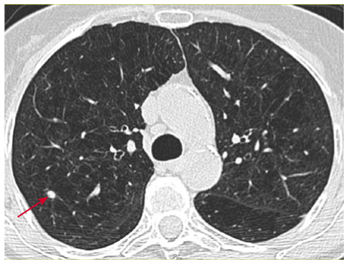
The goal of this challenge is to develop new methods to predict survival time of patients diagnosed with lung cancer, based 3-dimensional radiology images (Computed Tomography scanner). Radiology data refers to various kinds of imaging modalities such as MRI, Echography or CT scans. In a clinical context, such modalities are very valuable because, unlike biopsies, those images are non invasive​: the pathology and the patient’s body remain untouched. Furthermore, those are much cheaper to operate and can, hence, be acquired at multiple timepoints and be used to track the disease through time. CT scan is a widely spread and popular exam in oncology: it reflects the density of the tissues of the human body. It is, then, adapted to the study of lung cancer because lungs are mostly filled with air (low density) while tumors are made of dense tissues.



Lung Cancer is one of the most represented cancer type (around 230.000 cases per year in the US) among which 80% are identified as Non Small Cell Lung Cancer (NSCLC). This subtype of lung cancer is characterized by peculiarly large tumors, hence called masses​, which can occupy significant portions of the total lung volumes, involving serious threats to the patient’s breathing abilities. Non Small Cell Lung Cancer can itself be split into four major subtypes based on histology observations: squamous cell carcinoma, large cell carcinoma, adenocarcinoma and a mixture of all.



When assessing the disease, radiologists will, among other aspects, look at the evolution through time of morphological features such as the gross tumour volume. However, being able to predict the survival of a patient from a single time point would be highly valuable as it would help in identifying prognostic features from radiology images, in addition to bringing valuable information at a low price in clinical trials. Features can be here understood as a very broad term which can refer to various characteristics of the tumor environment, such as its size, the density of the tumor, or even textural information extracted from the tumor zone. Designing those ​features​ requires advanced medical knowledge, and a lot of experience in prognosis / medical models. Hence, a large number of informative features have been identified by groups of medical experts in radio-oncology, related to colour or density heterogeneity, compactness, and many others.

Challenge goals

Goal

Data description

Data

Labels

Inputs

For each patient, we provided four inputs:

1. Images (one scan and one mask per patient): we furnish crops of both the scan and the mask, centered around the tumor region. Those crops are of fixed 92^3 mm^3 size.
2. Radiomics features (an ensemble of 53 quantitative features per patient, extracted from the scan).
3. Clinical data

Images

import numpy as np
archive = np.load('patient_000.npz')
scan = archive['scan']
mask = archive['mask']
# scan.shape equals mask.shape

Radiomics features

Clinical data

Outputs

import pandas as pd
train_output = pd.read_csv( 'train/output.csv', index_col=0)
p0 = train_output.loc[202]
print(p0.Event) # prints 1 or 0
print(p0.SurvivalTime)
# prints time to event (time to death or time to last known alive) in days

1. Training set (70%)
2. Public test set (15%)
3. Private test set (15%)

In total the training set contains

Benchmark description

Baseline model for survival regression on NSCLC clinical data

Model

Baseline hazard

The model is a Cox proportional hazard (Cox-PH) model (see this description of the Cox proportional hazards model).
The model regresses the proportional risk (individual risk factor) of each patient in the dataset, based on the TNM staging (see wikipedia) of this patient at t=0. The proportional risk at time $t$ is formulated as follows:

$$h(t|x)=h_0(t) e^{\beta^T x}$$

where $h_0(t)$ is the baseline proportional risk factor, $x$ is a vector of covariates, and $\beta$ is the vector of fitted coefficients whose entries measure the impact of each covariate on the survival function.
A positive coefficient $\beta_k$ indicates a worse prognosis and a negative coefficient indicates a protective effect of the variable $x_k$ with which it is associated. They are the parameters one wants to find.

Hazard ratio

The effects of covariates does not change over time, only the baseline hazard function does. It is the non parametric part of the model, it can take any form. However it vanishes when we take the ratio of hazards between two patients. The hazard ratio measures which patient is the most at risk and is constant over time (hence proportional hazards). Indeed, by taking the ratio of hazard functions of two patients, the baseline hazard $h_0(t)$ vanishes :

$$\frac{h(t|x_i)}{h(t|x_j)}=e^{\beta^T (x_i - x_j)}$$

Data

This baseline is trained on a selection of features from both clinical data file and radiomics file. A Cox-PH model was fitted on

1. Tumor sphericity, a measure of the roundness of the shape of the tumor region relative to a sphere, regardless its dimensions (size).
2. The tumor's surface to volume ratio is a measure of the compactness of the tumor, related to its size.
3. The tumor's maximum 3d diameter The biggest diameter measurable from the tumor volume
4. The dataset of origin
5. The N-tumoral stage grading of the tumor describing nearby (regional) lymph nodes involved
6. The tumor's joint entropy, specifying the randomness in the image pixel values
7. The tumor's inverse different, a measure of the local homogeneity of the tumor
8. The tumor's inverse difference moment is another measurement of the local homogeneity of the tumor

A finer definition of those features can be found here

Performances

The baseline proposed reaches a Concordance Index (CI) of 0.691 on the public test set.

Metric

The concordance index (C-index) is a generalization of the Area Under the Curve (or AUC) which can take into account censored data. This metric is commonly used to evaluate and compare predictive models with censored data. The C-index evaluates whether predicted survival times are ranked in the same order as their true survival time. Indeed because of censored data, the actual ordering of patient survival is not always available. A pair of patient is said “admissible” if patients can be ordered. The pair $(i, j)$ is admissible if patients $i$ and $j$ are not censored, or if patient $i$ dies at $t = k$ and patient $j$ is censored at $t > k$. On the contrary, if both patients are censored or if patient $i$ died at $t = k′$ and patient $j$ is censored at $t < k′$, the pair is not admissible. Indeed in that last case, patient $j$ may or may not have died before $k’$.

The C-index is then defined as follows:

$$\mathrm{C}_{\mathrm{index}}=\frac{\text{Number of concordant pairs}}{\text{Number of admissible pairs}}$$

Note that the C-index does not compare absolute predicted survival times like usual regression metrics, but only relative survival times, by comparing ordering of the predictions and ordering of the true survival times.